Code Example
This notebook contains a demo of the IVIM fitting approach proposed in "Deep Learning How to Fit an Intravoxel Incoherent Motion Model to Diffusion-Weighted MRI" by Barbieri et al., 2019. A preprint of the paper can be found at: https://arxiv.org/abs/1903.00095
Start by creating some training data.
Please note:
- The creation of a separate training dataset is only necessary for the purpose of this notebook.
- In an actual clinical study, the network would be trained on voxels from the set of clinical images of interest. Take care to:
- Exclude background voxels.
- Normalize by the b=0 value (this is not stricly necessary but should facilitate training).
# import libraries
import numpy as np
import matplotlib.pyplot as plt
import torch
import torch.nn as nn
import torch.optim as optim
import torch.utils.data as utils
from tqdm import tqdm
# define ivim function
def ivim(b, Dp, Dt, Fp):
    return Fp*np.exp(-b*Dp) + (1-Fp)*np.exp(-b*Dt)
# define b values
b_values = np.array([0,10,20,60,150,300,500,1000])
# training data
num_samples = 100000
X_train = np.zeros((num_samples, len(b_values)))
for i in range(len(X_train)):
    Dp = np.random.uniform(0.01, 0.1)
    Dt = np.random.uniform(0.0005, 0.002)
    Fp = np.random.uniform(0.1, 0.4)
    X_train[i, :] = ivim(b_values, Dp, Dt, Fp)
# add some noise
X_train_real = X_train + np.random.normal(scale=0.01, size=(num_samples, len(b_values)))
X_train_imag = np.random.normal(scale=0.01, size=(num_samples, len(b_values)))
X_train = np.sqrt(X_train_real**2 + X_train_imag**2)
Let's create the neural network class and instantiate it.
class Net(nn.Module):
    def __init__(self, b_values_no0):
        super(Net, self).__init__()

        self.b_values_no0 = b_values_no0
        self.fc_layers = nn.ModuleList()
        for i in range(3): # 3 fully connected hidden layers
            self.fc_layers.extend([nn.Linear(len(b_values_no0), len(b_values_no0)), nn.ELU()])
        self.encoder = nn.Sequential(*self.fc_layers, nn.Linear(len(b_values_no0), 3))

    def forward(self, X):
        params = torch.abs(self.encoder(X)) # Dp, Dt, Fp
        Dp = params[:, 0].unsqueeze(1)
        Dt = params[:, 1].unsqueeze(1)
        Fp = params[:, 2].unsqueeze(1)

        X = Fp*torch.exp(-self.b_values_no0*Dp) + (1-Fp)*torch.exp(-self.b_values_no0*Dt)

        return X, Dp, Dt, Fp
# Network
b_values_no0 = torch.FloatTensor(b_values[1:])
net = Net(b_values_no0)

# Loss function and optimizer
criterion = nn.MSELoss()
optimizer = optim.Adam(net.parameters(), lr = 0.001)
Create batch queues.
batch_size = 128
num_batches = len(X_train) // batch_size
X_train = X_train[:,1:] # exlude the b=0 value as signals are normalized
trainloader = utils.DataLoader(torch.from_numpy(X_train.astype(np.float32)),
                                batch_size = batch_size,
                                shuffle = True,
                                num_workers = 2,
                                drop_last = True)
Train, this might take a few minutes.
# Best loss
best = 1e16
num_bad_epochs = 0
patience = 10

# Train
for epoch in range(1000):
    print("-----------------------------------------------------------------")
    print("Epoch: {}; Bad epochs: {}".format(epoch, num_bad_epochs))
    net.train()
    running_loss = 0.

    for i, X_batch in enumerate(tqdm(trainloader), 0):
        # zero the parameter gradients
        optimizer.zero_grad()

        # forward + backward + optimize
        X_pred, Dp_pred, Dt_pred, Fp_pred = net(X_batch)
        loss = criterion(X_pred, X_batch)
        loss.backward()
        optimizer.step()
        running_loss += loss.item()

    print("Loss: {}".format(running_loss))
    # early stopping
    if running_loss < best:
        print("############### Saving good model ###############################")
        final_model = net.state_dict()
        best = running_loss
        num_bad_epochs = 0
    else:
        num_bad_epochs = num_bad_epochs + 1
        if num_bad_epochs == patience:
            print("Done, best loss: {}".format(best))
            break
print("Done")
# Restore best model
net.load_state_dict(final_model)
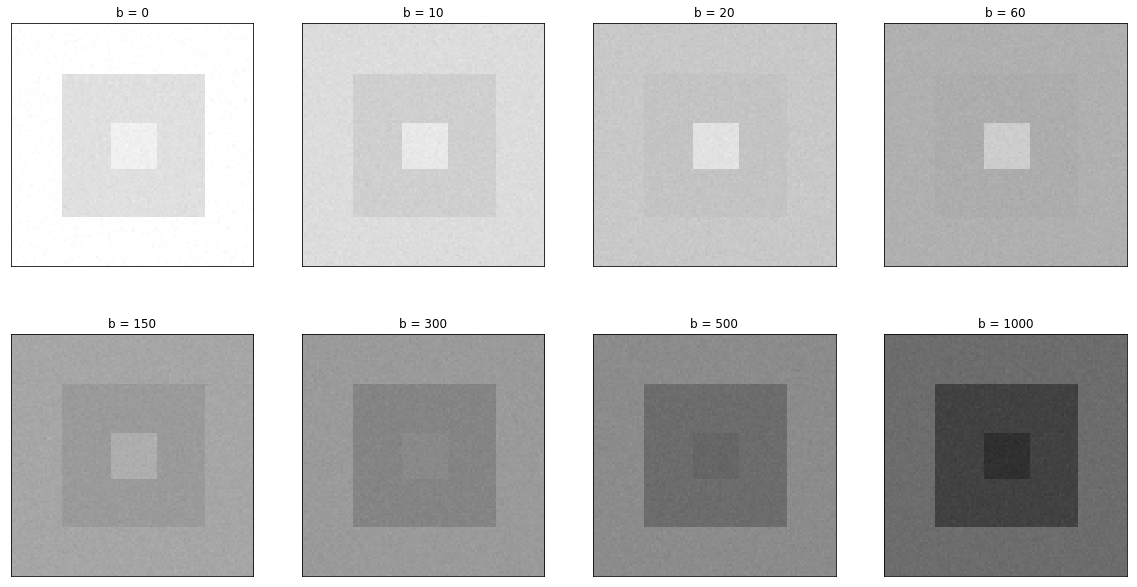
Create a simulated diffusion-weighted image. The image contains three regions with different Dp, Dt, and Fp values.
# define parameter values in the three regions
S0_region0, S0_region1, S0_region2 = 1500, 1400, 1600
Dp_region0, Dp_region1, Dp_region2 = 0.02, 0.04, 0.06
Dt_region0, Dt_region1, Dt_region2 = 0.0015, 0.0010, 0.0005
Fp_region0, Fp_region1, Fp_region2 = 0.1, 0.2, 0.3
# image size
sx, sy, sb = 100, 100, len(b_values)
# create image
dwi_image = np.zeros((sx, sy, sb))
Dp_truth = np.zeros((sx, sy))
Dt_truth = np.zeros((sx, sy))
Fp_truth = np.zeros((sx, sy))

# fill image with simulated values
for i in range(sx):
    for j in range(sy):
        if (40 < i < 60) and (40 < j < 60):
            # region 0
            dwi_image[i, j, :] = S0_region0*ivim(b_values, Dp_region0, Dt_region0, Fp_region0)
            Dp_truth[i, j], Dt_truth[i, j], Fp_truth[i, j] = Dp_region0, Dt_region0, Fp_region0
        elif (20 < i < 80) and (20 < j < 80):
            # region 1
            dwi_image[i, j, :] = S0_region1*ivim(b_values, Dp_region1, Dt_region1, Fp_region1)
            Dp_truth[i, j], Dt_truth[i, j], Fp_truth[i, j] = Dp_region1, Dt_region1, Fp_region1
        else:
            # region 2
            dwi_image[i, j, :] = S0_region2*ivim(b_values, Dp_region2, Dt_region2, Fp_region2)
            Dp_truth[i, j], Dt_truth[i, j], Fp_truth[i, j] = Dp_region2, Dt_region2, Fp_region2
# add some noise
dwi_image_real = dwi_image + np.random.normal(scale=15, size=(sx, sy, sb))
dwi_image_imag = np.random.normal(scale=15, size=(sx, sy, sb))
dwi_image = np.sqrt(dwi_image_real**2 + dwi_image_imag**2)
# plot simulated diffusion weighted image
fig, ax = plt.subplots(2, 4, figsize=(20,20))
b_id = 0
for i in range(2):
    for j in range(4):
        ax[i, j].imshow(dwi_image[:, :, b_id], cmap='gray', clim=(0, 1600))
        ax[i, j].set_title('b = ' + str(b_values[b_id]))
        ax[i, j].set_xticks([])
        ax[i, j].set_yticks([])
        b_id += 1
plt.subplots_adjust(hspace=-0.6)
plt.show()
Estimate IVIM parameter values for the simulated image.
# normalize signal
dwi_image_long = np.reshape(dwi_image, (sx*sy, sb))
S0 = np.expand_dims(dwi_image_long[:,0], axis=-1)
dwi_image_long = dwi_image_long[:,1:]/S0

net.eval()
with torch.no_grad():
    _, Dp, Dt, Fp = net(torch.from_numpy(dwi_image_long.astype(np.float32)))

Dp = Dp.numpy()
Dt = Dt.numpy()
Fp = Fp.numpy()

# make sure Dp is the larger value between Dp and Dt
if np.mean(Dp) < np.mean(Dt):
    Dp, Dt = Dt, Dp
    Fp = 1 - Fp
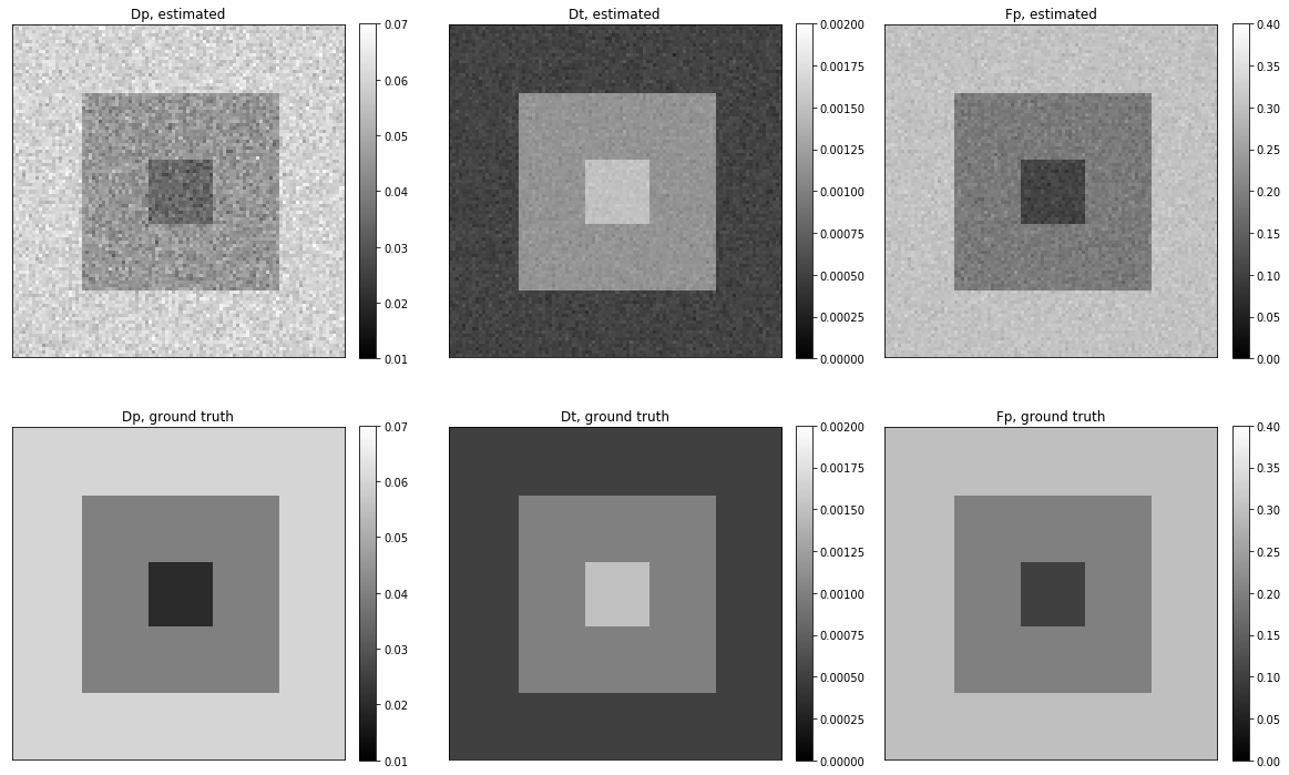
Plot parameter estimates and corresponding ground truths.
fig, ax = plt.subplots(2, 3, figsize=(20,20))

Dp_plot = ax[0,0].imshow(np.reshape(Dp, (sx, sy)), cmap='gray', clim=(0.01, 0.07))
ax[0,0].set_title('Dp, estimated')
ax[0,0].set_xticks([])
ax[0,0].set_yticks([])
fig.colorbar(Dp_plot, ax=ax[0,0], fraction=0.046, pad=0.04)

Dp_t_plot = ax[1,0].imshow(Dp_truth, cmap='gray', clim=(0.01, 0.07))
ax[1,0].set_title('Dp, ground truth')
ax[1,0].set_xticks([])
ax[1,0].set_yticks([])
fig.colorbar(Dp_t_plot, ax=ax[1,0], fraction=0.046, pad=0.04)

Dt_plot = ax[0,1].imshow(np.reshape(Dt, (sx, sy)), cmap='gray', clim=(0, 0.002))
ax[0,1].set_title('Dt, estimated')
ax[0,1].set_xticks([])
ax[0,1].set_yticks([])
fig.colorbar(Dt_plot, ax=ax[0,1],fraction=0.046, pad=0.04)

Dt_t_plot = ax[1,1].imshow(Dt_truth, cmap='gray', clim=(0, 0.002))
ax[1,1].set_title('Dt, ground truth')
ax[1,1].set_xticks([])
ax[1,1].set_yticks([])
fig.colorbar(Dt_t_plot, ax=ax[1,1], fraction=0.046, pad=0.04)

Fp_plot = ax[0,2].imshow(np.reshape(Fp, (sx, sy)), cmap='gray', clim=(0, 0.4))
ax[0,2].set_title('Fp, estimated')
ax[0,2].set_xticks([])
ax[0,2].set_yticks([])
fig.colorbar(Fp_plot, ax=ax[0,2],fraction=0.046, pad=0.04)

Fp_t_plot = ax[1,2].imshow(Fp_truth, cmap='gray', clim=(0, 0.4))
ax[1,2].set_title('Fp, ground truth')
ax[1,2].set_xticks([])
ax[1,2].set_yticks([])
fig.colorbar(Fp_t_plot, ax=ax[1,2], fraction=0.046, pad=0.04)

plt.subplots_adjust(hspace=-0.5)
plt.show()